import TutorialWorld.Level1
import TutorialWorld.Level2
import TutorialWorld.Level3
import TutorialWorld.Level4

Natural Numbers Tutorial

This tutorial is based on the Natural Number Game by Kevin Buzzard and Mohammad Pedramfar.

This tutorial provides the same content in a book format that is designed to be read online or run in your local Visual Studio Code with the Lean4 "extension". The extension will install the Lean4 compiler and language service for you so it is easy to setup - see the Quick Start for more information.

To run this tutorial in Visual Studio Code, first clone the https://github.com/leanprover/lean4-samples repo. Then you must open the NaturalNumbers folder in Visual Studio Code using File/Open folder in order for it to function correctly.

How to use this sample

When reading this content in a web browser the code samples are annotated with type information and you can see the proof tactic state by hovering your mouse over these little bubbles that look like this:

When viewing this content in Visual Studio Code you will find this tactic state information in the Lean extension "Info View" panel.

This sample is organized into sections called "worlds" and each section has a sequential set of learning levels. The idea is that you should work through the worlds and levels in order. Each level has a description of the goal and a set of tasks to complete.

In this sample you will not use the built in support for natural numbers in Lean because that would be too easy. You will start from scratch defining your own new type called MyNat. Your version of the natural numbers will satisfy something called the principle of mathematical induction, and a couple of other things too (Peano's axioms). Since you are starting from scratch, you will have to prove all the basic theorems about your numbers like x + y = y + x and so on. This is your job. You're going to prove mathematical theorems using the Lean theorem prover.

You're going to prove these theorems using tactics. The introductory world, Tutorial World, will take you through some of these tactics. During your proofs, your "goal" (i.e. what you're supposed to be proving) will be displayed in the Visual Studio Code InfoView with a ⊢ symbol in front of it. If the InfoView says "Goals accomplished 🎉", you have closed all the goals in the level and can move on to the next level in the world you're in.

You are now ready to dive into Tutorial World: Level 1.

There is also an "online" version under development that works with Lean 4, see https://github.com/PatrickMassot/NNG4.

If you want to see the original "Lean 3" game version of this content, go to https://github.com/ImperialCollegeLondon/natural_number_game which is also hosted in this online version.

import MyNat.Definition
namespace MyNat

Tutorial world

Level 1: the rfl tactic

Let's learn some tactics! Let's start with the rfl tactic. rfl stands for "reflexivity", which is a fancy way of saying that it will prove any goal of the form A = A. It doesn't matter how complicated A is, all that matters is that the left hand side is exactly equal to the right hand side (a computer scientist would say "definitionally equal"). I really mean "press the same buttons on your computer in the same order" equal. For example, x * y + z = x * y + z can be proved by rfl, but x + y = y + x cannot.

Each level in this world involves proving a theorem or a lemma (a lemma is just a baby theorem). The goal of the theorem will be a mathematical statement with a ⊢ just before it. We will use tactics to manipulate and ultimately close (i.e. prove) these goals.

Note that while lean4 does not define the keyword lemma it has been added to the mathlib4 library so it is coming from the import Mathlib.Tactic.Basic that is included in MyNat.Definition.

Let's see rfl in action! At the bottom of the text in this box, there's a lemma, which says that if x, y and z are natural numbers then xy + z = xy + z. Locate this lemma (if you can't see the lemma and these instructions at the same time, make this box wider by dragging the sides). Let's supply the proof. Click on the word sorry and then delete it. When the system finishes being busy, you'll be able to see your goal in the Visual Studio Code InfoView.

Remember that the goal is the thing with the unicode symbol ⊢ just before it. The goal in this case is x * y + z = x * y + z, where x, y and z are some of your very own natural numbers. That's a pretty easy goal to prove -- you can just prove it with the rfl tactic. Where it used to say sorry, write rfl.

Lemma

For all natural numbers x, y and z, we have xy + z = xy + z.

lemma 
example1: ∀ (x y z : MyNat), x * y + z = x * y + z
example1 (
x: MyNat
x 
y: MyNat
y 
z: MyNat
z : 
MyNat: Type
MyNat) : 
x: MyNat
x * 
y: MyNat
y + 
z: MyNat
z = 
x: MyNat
x * 
y: MyNat
y + 
z: MyNat
z := by
x, y, z: MyNat
x * y + z = x * y + z
  rfl
Goals accomplished! 🐙

If all goes well Lean will print Goals accomplished 🎉 in the InfoView. You just did the first level of the tutorial!

For each level, the idea is to get Lean into this state: with the InfoView saying "Goals accomplished 🎉" when the cursor is placed at the end of the line that completes the proof.

If you want to be reminded about the rfl tactic, you can hover the mouse over the rfl keyword and a tooltip will appear with information about this tactic. You can also press F12 to jump to the definition of that tactic were there will be lots more handy information. We have also included a Tactics Section that lists all the tactics we use in this tutorial.

Now click on "next level" in the top right of your browser to go onto the second level of tutorial world, where we'll learn about the rw tactic.

Now you are ready for Level2.lean.

import MyNat.Definition
namespace MyNat

Tutorial world

Level 2: The rewrite tactic

The rewrite tactic is the way to "substitute in" the value of a variable. In general, if you have a hypothesis of the form A = B, and your goal mentions the left hand side A somewhere, then the rewrite tactic will replace the A in your goal with a B. Below is a theorem which cannot be proved using rfl -- you need a rewrite first.

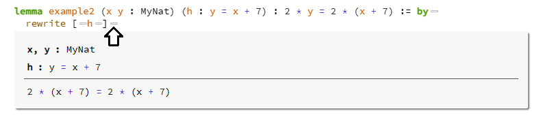
Take a look in the InfoView at what you have. The variables x and y are natural numbers, and there is a proof h that y = x + 7. Your goal then is to prove that 2y = 2(x + 7). This goal is obvious -- you just substitute in y = x + 7 and you're done. In Lean, you do this substitution using the rewrite tactic.

Lemma

If x and y are natural numbers, and y = x + 7, then 2y = 2(x + 7).

lemma 
example2: ∀ (x y : MyNat), y = x + 7 → 2 * y = 2 * (x + 7)
example2 (
x: MyNat
x 
y: MyNat
y : 
MyNat: Type
MyNat) (
h: y = x + 7
h : 
y: MyNat
y = 
x: MyNat
x + 
7: MyNat
7) : 
2: MyNat
2 * 
y: MyNat
y = 
2: MyNat
2 * (
x: MyNat
x + 
7: MyNat
7) := by
x, y: MyNat
h: y = x + 7
2 * y = 2 * (x + 7)
  rewrite [
x, y: MyNat
h: y = x + 7
2 * y = 2 * (x + 7)
h: y = x + 7
h
x, y: MyNat
h: y = x + 7
2 * (x + 7) = 2 * (x + 7)]
x, y: MyNat
h: y = x + 7
2 * (x + 7) = 2 * (x + 7)
  rfl
Goals accomplished! 🐙

Did you see what happened to the goal? (Put your cursor at the end of the rewrite line). The goal doesn't close, but it changes from ⊢ 2 * y = 2 * (x + 7) to ⊢ 2 * (x + 7) = 2 * (x + 7). And since these are now identical you can just close this goal with rfl.

You should now see "Goals accomplished 🎉" (with cursor at the end of the rfl line). The square brackets here is a List object because rewrite can rewrite using multiple hypotheses in sequence.

If you are reading this book online you can move the mouse over each bubble that is added to the end of each line (that look like this: ) to see what the tactic state is at that point in the proof.

The other way you know the goal is complete is to look a the Visual Studio Code Problems list window, if there are no error saying "unsolved goals" then you are done.

The documentation for rewrite will appear when you hover the mouse over it. We have also included a Tactics Section that lists all the tactics we use in this tutorial.

Now, Lean has another similar tactic named rw which does both the rewrite and the rfl. Try changing to rw above and you will see the rfl is no longer needed.

Details

Now you are ready for Level3.lean.

import MyNat.Definition
namespace MyNat
open MyNat

Tutorial world

Level 3: Peano's axioms.

The import above gives us the type MyNat of natural numbers. But it also gives us some other things, which we'll take a look at now:

• a term (0 : MyNat), interpreted as the MyNat.zero.
• a function succ : MyNat → MyNat, with succ n interpreted as "the number after n", or the successor of n.
• The principle of mathematical induction.

These axioms are essentially the axioms isolated by Peano which uniquely characterize the natural numbers (you also need recursion, but you can ignore it for now). The first axiom says that 0 is a natural number. The second says that there is a succ function which eats a number and spits out the number after it, so succ 0 = 1, succ 1 = 2, and so on.

Peano's last axiom is the principle of mathematical induction. This is a deeper fact. It says that if you have infinitely many true/false statements P(0), P(1), P(2), and so on, and if P(0) is true, and if for every natural number d you know that P(d) implies P(succ d), then P(n) must be true for every natural number n. It's like saying that if you have a long line of dominoes, and if you knock the first one down, and if you know that if a domino falls down then the one after it will fall down too, then you can deduce that all the dominos will fall down. You can also think of it as saying that every natural number can be built by starting at 0 and then applying succ a finite number of times.

Peano's insights were firstly that these axioms completely characterise the natural numbers, and secondly that these axioms alone can be used to build a whole bunch of other structure on the natural numbers, for example addition, multiplication and so on.

This world is all about seeing how far these axioms of Peano can take us.

Let's practice your use of the rewrite tactic in the following example. The hypothesis h is a proof that succ a = b and you want to prove that succ (succ a) = succ b. In words, you're going to prove that if b is the number after a then succ b is the number after succ a. Now here's a tricky question. If your goal is ⊢ succ (succ a) = succ b, and your hypothesis is h : succ a = b, then what will the goal change to when we type rewrite [h]?

Lemma

If succ a = b, then succ (succ a) = succ b.

lemma 
example3: ∀ (a b : MyNat), succ a = b → succ (succ a) = succ b
example3 (
a: MyNat
a 
b: MyNat
b : 
MyNat: Type
MyNat) (
h: succ a = b
h : (
succ: MyNat → MyNat
succ 
a: MyNat
a) = 
b: MyNat
b) : 
succ: MyNat → MyNat
succ (
succ: MyNat → MyNat
succ 
a: MyNat
a) = 
succ: MyNat → MyNat
succ 
b: MyNat
b := by
a, b: MyNat
h: succ a = b
succ (succ a) = succ b
  rewrite [
a, b: MyNat
h: succ a = b
succ (succ a) = succ b
h: succ a = b
h
a, b: MyNat
h: succ a = b
succ b = succ b]
a, b: MyNat
h: succ a = b
succ b = succ b
  rfl
Goals accomplished! 🐙

Remember that rewrite [h] will look for the left hand side of h in the goal, and will replace it with the right hand side. Try and figure out how the goal will change, and then try it.

The answer: Lean changed succ a into b, so the goal became succ b = succ b. That goal is of the form X = X, so you can complete prove the proof using rfl which rw does for you.

Important note : the tactic rewrite expects a proof afterwards (e.g. rewrite [h1]). But rfl is just rfl.

You may be wondering whether you could have just substituted in the definition of b and proved the goal that way. To do that, you would want to replace the right hand side of h with the left hand side. You do this in Lean by writing rw [← h]. You get the left-arrow by typing \l and then a space; note that this is a small letter L, not a number 1. You can just edit your proof and try it.

You may also be wondering why we keep writing succ b instead of b + 1. This is because we haven't defined addition yet! On the next level, the final level of Tutorial World, we will introduce addition, and then you'll be ready to enter Addition World.

Now you are ready for Level4.lean.

import MyNat.Addition
namespace MyNat
open MyNat

Tutorial world

Level 4: addition

We have a new import -- the definition of addition.

Peano defined addition a + b by induction on b, or, more precisely, by recursion on b. He first explained how to add 0 to a number: this is the base case.

• add_zero (a : MyNat) : a + 0 = a

We will call this theorem add_zero. More precisely, add_zero is the name of the proof of the theorem. Note the name of this proof. Mathematicians sometimes call it "Lemma 2.1" or "Hypothesis P6" or something. But computer scientists call it add_zero because it tells you what the answer to "x add zero" is. It's a much better name than "Lemma 2.1". Even better, you can use the rewrite tactic with add_zero. If you ever see x + 0 in your goal, rewrite [add_zero] should simplify it to x. This is because add_zero is a proof that x + 0 = x (more precisely, add_zero x is a proof that x + 0 = x but Lean can figure out the x from the context).

Now here's the inductive step. If you know how to add d to a, then Peano tells you how to add succ d to a. It looks like this:

• add_succ (a d : MyNat) : a + (succ d) = succ (a + d)

What's going on here is that we assume a + d is already defined, and we define a + (succ d) to be the number after it. Note the name of this proof too -- add_succ tells you how to add a successor to something. If you ever see ... + succ ... in your goal, you should be able to use rewrite [add_succ], to make progress.

Lemma`

For all natural numbers a, we have a + (succ 0) = succ a`.

lemma 
add_succ_zero: ∀ (a : MyNat), a + succ 0 = succ a
add_succ_zero (
a: MyNat
a : 
MyNat: Type
MyNat) : 
a: MyNat
a + (
succ: MyNat → MyNat
succ 
0: MyNat
0) = 
succ: MyNat → MyNat
succ 
a: MyNat
a := by
a: MyNat
a + succ 0 = succ a
  rewrite [
a: MyNat
a + succ 0 = succ a
add_succ: ∀ (a d : MyNat), a + succ d = succ (a + d)
add_succ
a: MyNat
succ (a + 0) = succ a]
a: MyNat
succ (a + 0) = succ a
  rewrite [
a: MyNat
succ (a + 0) = succ a
add_zero: ∀ (a : MyNat), a + 0 = a
add_zero
a: MyNat
succ a = succ a]
a: MyNat
succ a = succ a
  rfl
Goals accomplished! 🐙

Do you see that the goal at the end of the first rewrite now mentions ... + 0 ...? So this matches the add_zero theorem so you can now add the rewrite [add_zero].

After the rfl the proof is now complete: "Goals accomplished 🎉". Note that because rewrite takes a list, you can also write the above two lines in one using rewrite [add_succ, add_zero].

And remember rw also does rfl, you can replace the whole proof with rw [add_succ, add_zero].

Examining proofs.

You might want to review this proof now; at three lines long it is your current record. Don't worry there are much longer proofs, in fact, the Liquid Tensor Experiment contains 90,000 lines of Lean proofs! For this reason Lean is a real programming language with support for abstraction and extension so that you can get as much reusability as possible in your Lean code.

The easiest way to see how the proof goal state progresses is to place your cursor at the beginning of each line using the Up/Down arrow key to move down the proof and see the effect of the previous line on the goal shown in the InfoView.

Next

You have finished tutorial world! When you're happy, please move onto Addition World, and learn about proof by induction.

Troubleshooting

Question: why has the InfoView gone blank?

Answer: try placing the cursor at different places in the file, the InfoView shows the context at the cursor location. If the InfoView is not updating at all no matter what you do then there might be a problem with your VS Code setup. See the Quick Start for more information.

import AdditionWorld.Level1
import AdditionWorld.Level2
import AdditionWorld.Level3
import AdditionWorld.Level4
import AdditionWorld.Level5
import AdditionWorld.Level6

Addition World.

Welcome to Addition World. If you've done all four levels in Tutorial World and know about rewrite, rw and rfl, then you're in the right place. We'll use rw from her on out just for convenience. Here's a reminder of the things you're now equipped with which we'll need in this world.

Data:

• a type called MyNat
• a term (0 : MyNat), interpreted as the number zero.
• a function succ : MyNat → MyNat, with succ n interpreted as "the number after n".
• Usual numerical notation 0,1,2 etc (although 2 onwards will be of no use to us until much later ;-) ).
• Addition (with notation a + b).

Theorems:

• add_zero (a : MyNat) : a + 0 = a. Use with rw [add_zero].
• add_succ (a b : MyNat) : a + succ b = succ (a + b). Use with rw [add_succ].
• The principle of mathematical induction. Use with induction (see below)

Tactics:

• rfl : proves goals of the form X = X
• rw [h] : if h is a proof of A = B, changes all A's in the goal to B's.
• induction n with ... : we're going to learn this right now.

Important thing

This is a really good time to check you can get "mouse hover help on anything in the Lean program. If you hover over 'rfl' you get information on that tactic. You can also press F12 to jump right into the definition of all the helpers functions we use here.

On to Addition World Level 1.

import MyNat.Addition -- imports addition.
namespace MyNat
open MyNat

Addition World.

Level 1: the induction tactic.

OK so let's see induction in action. We're going to prove

zero_add (n : MyNat) : 0 + n = n.

That is: for all natural numbers n, 0+n=n. Wait - what is going on here? Didn't you already prove that adding zero to n gave us n? No you didn't! You proved n + 0 = n, and that proof was called add_zero. We're now trying to establish zero_add, the proof that 0 + n = n. But aren't these two theorems the same? No they're not! It is true that x + y = y + x, but you haven't proved it yet, and in fact you will need both add_zero and zero_add in order to prove this. In fact x + y = y + x is the boss level for addition world, and induction is the only other tactic you'll need to beat it.

Now add_zero is one of Peano's axioms, so you don't need to prove it, you already have it (indeed, if you've used Goto Definition (F12) on this theorem you can even see it). To prove 0 + n = n we need to use induction on n. While we're here, note that zero_add is about zero add something, and add_zero is about something add zero. The names of the proofs tell you what the theorems are.

Lemma

For all natural numbers n, we have 0 + n = n.

lemma 
zero_add: ∀ (n : MyNat), 0 + n = n
zero_add (
n: MyNat
n : 
MyNat: Type
MyNat) : 
0: MyNat
0 + 
n: MyNat
n = 
n: MyNat
n := by
n: MyNat
0 + n = n
  induction 
n: MyNat
n with
n: MyNat
0 + n = n
  | 
zero: MyNat
zero =>
zero
0 + zero = zero rfl
Goals accomplished! 🐙
  | 
succ: MyNat → MyNat
succ 
n: MyNat
n 
ih: 0 + n = n
ih =>
n: MyNat
ih: 0 + n = n
succ
0 + succ n = succ n
      rw [
n: MyNat
ih: 0 + n = n
succ
0 + succ n = succ n
add_succ: ∀ (a d : MyNat), a + succ d = succ (a + d)
add_succ
n: MyNat
ih: 0 + n = n
succ
succ (0 + n) = succ n]
n: MyNat
ih: 0 + n = n
succ
succ (0 + n) = succ n
      rw [
n: MyNat
ih: 0 + n = n
succ
succ (0 + n) = succ n
ih: 0 + n = n
ih
n: MyNat
ih: 0 + n = n
succ
succ n = succ n]
Goals accomplished! 🐙

Notice that the induction tactic has created two sub-goals which you can match using vertical bar pattern patching.

The induction tactic has generated for us a base case with n = zero (the goal at the top) and an inductive step (the goal underneath). The golden rule: Tactics operate on the first goal

• the goal at the top. So let's just worry about that top goal now, the base case. If you place the cursor right after the => symbol you will see the goal listed in the InfoView as ⊢ 0 + zero = zero.

Remember that add_zero (the proof we have already) is the proof of x + 0 = x (for any x) so you can try rw [add_zero] here but what do you think the goal will change to? Remember to just keep focussing on the top goal, ignore the other one for now, it's not changing and in fact, the InfoView tells you why:

tactic 'rewrite' failed, did not find instance of the pattern in the target expression

But as you can see rfl can solve the first case. You should now see Goals accomplished 🎉 when your cursor is placed on the right of the rfl which means you have solved this base case sub-goal, and you are ready to tackle the next sub-goal -- the inductive step. Take a look at the text below the lemma to see an explanation of this goal.

In the successor case the InfoView tactic state should look something like this:

case succ
n: MyNat
ih: 0 + n = n
⊢ 0 + succ n = succ n

Important: make sure that you only have one goal at this point. You should have proved 0 + 0 = 0 by now. Tactics only operate on the top goal.

The first line just reminds you you're doing the inductive step. You have a fixed natural number n, and the inductive hypothesis ih : 0 + n = n which means this hypothesis proves 0 + n = n. Your goal is to prove 0 + succ n = succ n. In other words, we're showing that if the lemma is true for n, then it's also true for n + 1. That's the inductive step that you might be familiar with in proof by induction. Once we've proved this inductive step, you will have proved zero_add by the principle of mathematical induction.

To prove your goal, you need to use add_succ which you proved in Tutorial World Level 4. Note that add_succ 0 d is the result that 0 + succ d = succ (0 + d), so the first thing you need to do is to replace the left hand side 0 + succ d of your goal with the right hand side. You do this with the rw command: rw [add_succ] (or even rw [add_succ 0 n] if you want to give Lean all the inputs instead of making it figure them out itself). Notice goal changes to ⊢ succ (0 + n) = succ n.

Now remember the inductive hypothesis ih : 0 + d = d. This 0 + d matches the (0 + n) in the goal, so you can write that using rw [ih]. The goal will now change to

⊢ succ d = succ d

and the rw tactic will automatically finish our proof using the rfl tactic. After you apply it, Lean will inform you that there are no goals left. You are done!

Remember that you can write rw [add_succ, ih] also, but notice that rewriting is order dependent and that rw [ih, add_succ] does not work.

Now venture off on your own

Those three tactics --

• induction n with ...
• rw [h]
• rfl

will get you quite a long way through this tutorial. Using only these tactics do all of Addition World, all of Multiplication World including the boss level a * b = b * a, and even all of Power World including the fiendish final boss. This route will give you a good grounding in these three basic tactics; after that, if you are still interested, there are other worlds to master, where you can learn more tactics.

But we're getting ahead of ourselves, you still have to read the rest of Addition World. We're going to stop explaining stuff carefully now. If you get stuck or want to know more about Lean (e.g. how to do much harder maths in Lean), ask in #new members at the Lean chat. (login required, real name preferred, github account id is handy). Kevin or Mohammad or one of the other people there might be able to help.

On to level 2.

import MyNat.Addition -- imports addition.
namespace MyNat
open MyNat

Addition world

Level 2: add_assoc -- associativity of addition.

It's well-known that (1 + 2) + 3 = 1 + (2 + 3) -- if you have three numbers to add up, it doesn't matter which of the additions you do first. This fact is called associativity of addition by mathematicians, and it is not obvious. For example, subtraction really is not associative: (6 - 2) - 1 is really not equal to 6 - (2 - 1). We are going to have to prove that addition, as defined the way we've defined it, is associative.

To prove associativity of addition it is handy to recall that addition was defined by recursion on the right-most variable. This means you can use induction on the right-most variable (try other variables at your peril!). Note that when Lean writes a + b + c, it means (a + b) + c. If it wants to talk about a + (b + c) it will put the brackets in explicitly.

Reminder: you are done when you see "Goals accomplished 🎉" in the InfoView, and no errors in the VS Code Problems list.

Lemma

On the set of natural numbers, addition is associative. In other words, for all natural numbers a, b and c, we have (a + b) + c = a + (b + c).

lemma 
add_assoc: ∀ (a b c : MyNat), a + b + c = a + (b + c)
add_assoc (
a: MyNat
a 
b: MyNat
b 
c: MyNat
c : 
MyNat: Type
MyNat) : (
a: MyNat
a + 
b: MyNat
b) + 
c: MyNat
c = 
a: MyNat
a + (
b: MyNat
b + 
c: MyNat
c) := by
a, b, c: MyNat
a + b + c = a + (b + c)
  induction 
c: MyNat
c with
a, b, c: MyNat
a + b + c = a + (b + c)
  | 
zero: MyNat
zero =>
    -- ⊢ a + b + 0 = a + (b + 0)
a, b: MyNat
zero
a + b + zero = a + (b + zero)
    rw [
a, b: MyNat
zero
a + b + zero = a + (b + zero)
zero_is_0: zero = 0
zero_is_0
a, b: MyNat
zero
a + b + 0 = a + (b + 0)]
a, b: MyNat
zero
a + b + 0 = a + (b + 0)
    rw [
a, b: MyNat
zero
a + b + 0 = a + (b + 0)
add_zero: ∀ (a : MyNat), a + 0 = a
add_zero
a, b: MyNat
zero
a + b = a + (b + 0)]
a, b: MyNat
zero
a + b = a + (b + 0)
    rw [
a, b: MyNat
zero
a + b = a + (b + 0)
add_zero: ∀ (a : MyNat), a + 0 = a
add_zero
a, b: MyNat
zero
a + b = a + b]
Goals accomplished! 🐙
  | 
succ: MyNat → MyNat
succ 
c: MyNat
c 
ih: a + b + c = a + (b + c)
ih =>
    -- ⊢ (a + b) + succ d = a + (b + succ d)
a, b, c: MyNat
ih: a + b + c = a + (b + c)
succ
a + b + succ c = a + (b + succ c)
    rw [
a, b, c: MyNat
ih: a + b + c = a + (b + c)
succ
a + b + succ c = a + (b + succ c)
add_succ: ∀ (a d : MyNat), a + succ d = succ (a + d)
add_succ
a, b, c: MyNat
ih: a + b + c = a + (b + c)
succ
succ (a + b + c) = a + (b + succ c)]
a, b, c: MyNat
ih: a + b + c = a + (b + c)
succ
succ (a + b + c) = a + (b + succ c)
    rw [
a, b, c: MyNat
ih: a + b + c = a + (b + c)
succ
succ (a + b + c) = a + (b + succ c)
add_succ: ∀ (a d : MyNat), a + succ d = succ (a + d)
add_succ
a, b, c: MyNat
ih: a + b + c = a + (b + c)
succ
succ (a + b + c) = a + succ (b + c)]
a, b, c: MyNat
ih: a + b + c = a + (b + c)
succ
succ (a + b + c) = a + succ (b + c)
    rw [
a, b, c: MyNat
ih: a + b + c = a + (b + c)
succ
succ (a + b + c) = a + succ (b + c)
add_succ: ∀ (a d : MyNat), a + succ d = succ (a + d)
add_succ
a, b, c: MyNat
ih: a + b + c = a + (b + c)
succ
succ (a + b + c) = succ (a + (b + c))]
a, b, c: MyNat
ih: a + b + c = a + (b + c)
succ
succ (a + b + c) = succ (a + (b + c))
    rw [
a, b, c: MyNat
ih: a + b + c = a + (b + c)
succ
succ (a + b + c) = succ (a + (b + c))
ih: a + b + c = a + (b + c)
ih
a, b, c: MyNat
ih: a + b + c = a + (b + c)
succ
succ (a + (b + c)) = succ (a + (b + c))]
Goals accomplished! 🐙

On to Level 3.

import MyNat.Addition -- imports addition.
namespace MyNat
open MyNat

Addition World

Level 3: succ_add

Oh no! On the way to add_comm, a wild succ_add appears. succ_add is the proof that (succ a) + b = succ (a + b) for a and b in your natural number type. You need to prove this now, because you will need to use this result in our proof that a + b = b + a in the next level.

Think about why computer scientists called this result succ_add . There is a logic to all the names.

Note that if you want to be more precise about exactly where you want to rewrite something like add_succ (the proof you already have), you can do things like rw [add_succ (succ a)] or [rw add_succ (succ a) d], telling Lean explicitly what to use for the input variables for the function add_succ. Indeed, add_succ is a function -- it takes as input two variables a and b and outputs a proof that a + succ b = succ (a + b). The tactic rw [add_succ] just says to Lean "guess what the variables are".

Lemma

For all natural numbers a, b, we have (succ a) + b = succ (a + b).

lemma 
succ_add: ∀ (a b : MyNat), succ a + b = succ (a + b)
succ_add (
a: MyNat
a 
b: MyNat
b : 
MyNat: Type
MyNat) : 
succ: MyNat → MyNat
succ 
a: MyNat
a + 
b: MyNat
b = 
succ: MyNat → MyNat
succ (
a: MyNat
a + 
b: MyNat
b) := by
a, b: MyNat
succ a + b = succ (a + b)
  induction 
b: MyNat
b with
a, b: MyNat
succ a + b = succ (a + b)
  | 
zero: MyNat
zero =>
a: MyNat
zero
succ a + zero = succ (a + zero) rfl
Goals accomplished! 🐙
  | 
succ: MyNat → MyNat
succ 
b: MyNat
b 
ih: succ a + b = succ (a + b)
ih =>
a, b: MyNat
ih: succ a + b = succ (a + b)
succ
succ a + succ b = succ (a + succ b)
    rw [
a, b: MyNat
ih: succ a + b = succ (a + b)
succ
succ a + succ b = succ (a + succ b)
add_succ: ∀ (a d : MyNat), a + succ d = succ (a + d)
add_succ
a, b: MyNat
ih: succ a + b = succ (a + b)
succ
succ (succ a + b) = succ (a + succ b)]
a, b: MyNat
ih: succ a + b = succ (a + b)
succ
succ (succ a + b) = succ (a + succ b)
    rw [
a, b: MyNat
ih: succ a + b = succ (a + b)
succ
succ (succ a + b) = succ (a + succ b)
ih: succ a + b = succ (a + b)
ih
a, b: MyNat
ih: succ a + b = succ (a + b)
succ
succ (succ (a + b)) = succ (a + succ b)]
a, b: MyNat
ih: succ a + b = succ (a + b)
succ
succ (succ (a + b)) = succ (a + succ b)
    rw [
a, b: MyNat
ih: succ a + b = succ (a + b)
succ
succ (succ (a + b)) = succ (a + succ b)
add_succ: ∀ (a d : MyNat), a + succ d = succ (a + d)
add_succ
a, b: MyNat
ih: succ a + b = succ (a + b)
succ
succ (succ (a + b)) = succ (succ (a + b))]
Goals accomplished! 🐙

On to Level 4.

import MyNat.Addition -- imports addition.
import AdditionWorld.Level1 -- zero_add
import AdditionWorld.Level3 -- succ_add
namespace MyNat
open MyNat

Addition World

Level 4: add_comm

In this level, you'll prove that addition is commutative.

Lemma

On the set of natural numbers, addition is commutative. In other words, for all natural numbers a and b, we have a + b = b + a.

lemma 
add_comm: ∀ (a b : MyNat), a + b = b + a
add_comm (
a: MyNat
a 
b: MyNat
b : 
MyNat: Type
MyNat) : 
a: MyNat
a + 
b: MyNat
b = 
b: MyNat
b + 
a: MyNat
a := by
a, b: MyNat
a + b = b + a
  induction 
b: MyNat
b with
a, b: MyNat
a + b = b + a
  | 
zero: MyNat
zero =>
a: MyNat
zero
a + zero = zero + a
    rw [
a: MyNat
zero
a + zero = zero + a
zero_is_0: zero = 0
zero_is_0
a: MyNat
zero
a + 0 = 0 + a]
a: MyNat
zero
a + 0 = 0 + a
    rw [
a: MyNat
zero
a + 0 = 0 + a
add_zero: ∀ (a : MyNat), a + 0 = a
add_zero
a: MyNat
zero
a = 0 + a]
a: MyNat
zero
a = 0 + a
    rw [
a: MyNat
zero
a = 0 + a
zero_add: ∀ (n : MyNat), 0 + n = n
zero_add
a: MyNat
zero
a = a]
Goals accomplished! 🐙
  | 
succ: MyNat → MyNat
succ 
b: MyNat
b 
ih: a + b = b + a
ih =>
a, b: MyNat
ih: a + b = b + a
succ
a + succ b = succ b + a
    rw [
a, b: MyNat
ih: a + b = b + a
succ
a + succ b = succ b + a
add_succ: ∀ (a d : MyNat), a + succ d = succ (a + d)
add_succ
a, b: MyNat
ih: a + b = b + a
succ
succ (a + b) = succ b + a]
a, b: MyNat
ih: a + b = b + a
succ
succ (a + b) = succ b + a
    rw [
a, b: MyNat
ih: a + b = b + a
succ
succ (a + b) = succ b + a
ih: a + b = b + a
ih
a, b: MyNat
ih: a + b = b + a
succ
succ (b + a) = succ b + a]
a, b: MyNat
ih: a + b = b + a
succ
succ (b + a) = succ b + a
    rw [
a, b: MyNat
ih: a + b = b + a
succ
succ (b + a) = succ b + a
succ_add: ∀ (a b : MyNat), succ a + b = succ (a + b)
succ_add
a, b: MyNat
ih: a + b = b + a
succ
succ (b + a) = succ (b + a)]
Goals accomplished! 🐙

If you are keeping up so far then nice! You're nearly ready to make a choice: Multiplication World or Function World. But there are just a couple more useful lemmas in Addition World which you should prove first.

Press on to level 5.

import MyNat.Addition
namespace MyNat
open MyNat

Addition World

Level 5: succ_eq_add_one

axiom 
one_eq_succ_zero: 1 = succ 0
one_eq_succ_zero : (
1: MyNat
1 : 
MyNat: Type
MyNat) = 
MyNat.succ: MyNat → MyNat
MyNat.succ 
0: MyNat
0

We've just added one_eq_succ_zero (a statement that 1 = succ 0). This is not a proof it is an axiom. In Lean an axiom tells Lean don't both looking for a proof for this fact, just trust me, it's true. So you must be very careful in how you use axiom because it can lead to inconsistencies in subsequent proofs if your axiom contains an error.

Levels 5 and 6 are the two last levels in Addition World. Level 5 involves the number 1. When you see a 1 in your goal, you can write rw [one_eq_succ_zero] to get back to something which only mentions 0. This is a good move because 0 is easier for us to manipulate than 1 right now, because we have some theorems about 0 (zero_add, add_zero), but, other than 1 = succ 0, no theorems at all which mention 1. Let's prove one now.

Theorem

For any natural number n, we have succ n = n + 1.

theorem 
succ_eq_add_one: ∀ (n : MyNat), succ n = n + 1
succ_eq_add_one (
n: MyNat
n : 
MyNat: Type
MyNat) : 
succ: MyNat → MyNat
succ 
n: MyNat
n = 
n: MyNat
n + 
1: MyNat
1 := by
n: MyNat
succ n = n + 1
  rw [
n: MyNat
succ n = n + 1
one_eq_succ_zero: 1 = succ 0
one_eq_succ_zero
n: MyNat
succ n = n + succ 0]
n: MyNat
succ n = n + succ 0
  rw [
n: MyNat
succ n = n + succ 0
add_succ: ∀ (a d : MyNat), a + succ d = succ (a + d)
add_succ
n: MyNat
succ n = succ (n + 0)]
n: MyNat
succ n = succ (n + 0)
  rfl
Goals accomplished! 🐙

Note that lemma and theorem are the same thing and can be used interchangeably.

Hint: if you use proof by induction, but then find you don't need the hypothesis in the inductive step, then you probably didn't need proof by induction.

Press on to level 6.

import MyNat.Addition
import AdditionWorld.Level2 -- add_assoc
import AdditionWorld.Level4 -- add_comm
import AdditionWorld.Level5 -- succ_eq_add_one
namespace MyNat
open MyNat

Addition World

Level 6: add_right_comm

Lean sometimes writes a + b + c. What does it mean? The convention is that if there are no brackets displayed in an addition formula, the brackets are around the left most + (Lean's addition is "left associative"). So the goal in this level is (a + b) + c = (a + c) + b. This isn't quite add_assoc or add_comm, it's something you'll have to prove by putting these two theorems together.

If you hadn't picked up on this already, rw [add_assoc] will change (x + y) + z to x + (y + z), but to change it back you will need rw [← add_assoc]. Get the left arrow by typing \l then the space bar (note that this is L for left, not a number 1). Similarly, if h : a = b then rw [h] will change a's to b's and rw [← h] will change b's to a's.

Also, you can be (and will need to be, in this level) more precise about where to rewrite theorems. rw [add_comm] will just find the first ? + ? it sees and swap it around. You can target more specific additions like this: rw [add_comm a] will swap around additions of the form a + ?, and rw [add_comm a b] will only swap additions of the form a + b.

Where next?

There are thirteen more levels about addition after this one, but before you can attempt them you need to learn some more tactics. So after this level you have a choice -- either move on to Multiplication World (which you can solve with the tactics you know) or try Function World (and learn some new ones). Other things, perhaps of interest to some players, are mentioned below the lemma.

Lemma

For all natural numbers a, b and c, we have a + b + c = a + c + b.

lemma 
add_right_comm: ∀ (a b c : MyNat), a + b + c = a + c + b
add_right_comm (
a: MyNat
a 
b: MyNat
b 
c: MyNat
c : 
MyNat: Type
MyNat) : 
a: MyNat
a + 
b: MyNat
b + 
c: MyNat
c = 
a: MyNat
a + 
c: MyNat
c + 
b: MyNat
b := by
a, b, c: MyNat
a + b + c = a + c + b
  rw [
a, b, c: MyNat
a + b + c = a + c + b
add_assoc: ∀ (a b c : MyNat), a + b + c = a + (b + c)
add_assoc
a, b, c: MyNat
a + (b + c) = a + c + b]
a, b, c: MyNat
a + (b + c) = a + c + b
  rw [
a, b, c: MyNat
a + (b + c) = a + c + b
add_comm: ∀ (a b : MyNat), a + b = b + a
add_comm 
b: MyNat
b 
c: MyNat
c
a, b, c: MyNat
a + (c + b) = a + c + b]
a, b, c: MyNat
a + (c + b) = a + c + b
  rw [
a, b, c: MyNat
a + (c + b) = a + c + b←
add_assoc: ∀ (a b c : MyNat), a + b + c = a + (b + c)
add_assoc
a, b, c: MyNat
a + c + b = a + c + b]
Goals accomplished! 🐙

If you have got this far, then you have become very good at manipulating equalities in Lean. You can also now connect four handy type class instances to your MyNat type as follows:

-- instance : AddSemigroup MyNat where
--   add_assoc := add_assoc

-- instance : AddCommSemigroup MyNat where
--   add_comm := add_comm

-- instance : AddMonoid MyNat where
--   nsmul :=  λ x y => (myNatFromNat x) * y
--   nsmul_zero' := MyNat.zero_mul
--   nsmul_succ' n x := by
--     show ofNat (MyNat.succ n) * x = x + MyNat n * x
--     rw [MyNat.ofNat_succ, MyNat.add_mul, MyNat.add_comm, MyNat.one_mul]

-- instance : AddCommMonoid MyNat where
--   zero_add := zero_add
--   add_zero := add_zero
--   add_comm := add_comm
--   nsmul_zero' := ...
--   nsmul_succ' := ...

-- BUGBUG: really? These last two require theorems about multiplication?
-- like add_mul and zero_mul, which is dependent on mul_comm...?

In Multiplication World you will be able to collect such advanced collectibles as MyNat.comm_semiring and MyNat.distrib, and then move on to Power World and the famous collectible at the end of it.

One last thing -- didn't you think that solving this level add_right_comm was boring? Check out this AI that can do it for us.

The simp AI (it's just an advanced tactic really), and can nail some really tedious-for-a-human-to-solve goals. For example, check out this one-line proof. First you need to teach simp about the building blocks you have created so far:

lemma 
add_left_comm: ∀ (a b c : MyNat), a + (b + c) = b + (a + c)
add_left_comm (
a: MyNat
a 
b: MyNat
b 
c: MyNat
c : 
MyNat: Type
MyNat) : 
a: MyNat
a + (
b: MyNat
b + 
c: MyNat
c) = 
b: MyNat
b + (
a: MyNat
a + 
c: MyNat
c) := by
a, b, c: MyNat
a + (b + c) = b + (a + c)
  rw [
a, b, c: MyNat
a + (b + c) = b + (a + c)←
add_assoc: ∀ (a b c : MyNat), a + b + c = a + (b + c)
add_assoc
a, b, c: MyNat
a + b + c = b + (a + c)]
a, b, c: MyNat
a + b + c = b + (a + c)
  rw [
a, b, c: MyNat
a + b + c = b + (a + c)
add_comm: ∀ (a b : MyNat), a + b = b + a
add_comm 
a: MyNat
a
a, b, c: MyNat
b + a + c = b + (a + c)]
a, b, c: MyNat
b + a + c = b + (a + c)
  rw [
a, b, c: MyNat
b + a + c = b + (a + c)
add_assoc: ∀ (a b c : MyNat), a + b + c = a + (b + c)
add_assoc
a, b, c: MyNat
b + (a + c) = b + (a + c)]
Goals accomplished! 🐙

attribute [simp] 
add_assoc: ∀ (a b c : MyNat), a + b + c = a + (b + c)
add_assoc 
add_comm: ∀ (a b : MyNat), a + b = b + a
add_comm 
add_left_comm: ∀ (a b c : MyNat), a + (b + c) = b + (a + c)
add_left_comm

example: ∀ (a b c d e : MyNat), a + b + c + d + e = c + (b + e + a) + d
example (
a: MyNat
a 
b: MyNat
b 
c: MyNat
c 
d: MyNat
d 
e: MyNat
e : 
MyNat: Type
MyNat) :
  (((
a: MyNat
a+
b: MyNat
b)+
c: MyNat
c)+
d: MyNat
d)+
e: MyNat
e=(
c: MyNat
c+((
b: MyNat
b+
e: MyNat
e)+
a: MyNat
a))+
d: MyNat
d := by
a, b, c, d, e: MyNat
a + b + c + d + e = c + (b + e + a) + d
  simp
Goals accomplished! 🐙

Imagine having to do that one by hand! The AI closes the goal because it knows how to use associativity and commutativity sensibly in a commutative monoid.

For more info see the simp tactic.

You are now done with addition world. You can now decide whether to press on with Multiplication World and Power World (which can be solved with rw, rfl and induction), or to go on to Function World where you can learn the tactics needed to prove goals of the form P → Q, thus enabling you to solve more advanced addition world levels such as a + t = b + t → a = b. Note that Function World is more challenging mathematically; but if you can do Addition World you can surely do Multiplication World and Power World.

import MultiplicationWorld.Level1
import MultiplicationWorld.Level2
import MultiplicationWorld.Level3
import MultiplicationWorld.Level4
import MultiplicationWorld.Level5
import MultiplicationWorld.Level6
import MultiplicationWorld.Level7
import MultiplicationWorld.Level8
import MultiplicationWorld.Level9

Multiplication World

A new import import MyNat.Multiplication!

This import gives you the definition of multiplication on your natural numbers. It is defined by recursion, just like addition. Here are the two new axioms:

• mul_zero (a : MyNat) : a * 0 = 0
• mul_succ (a b : MyNat) : a * succ b = a * b + a

In words, we define multiplication by "induction on the second variable", with a * 0 defined to be 0 and, if we know a * b, then a times the number after b is defined to be a * b + a.

You can keep all the theorems you proved about addition, but for multiplication, those two results above are what you've got right now.

What's going on in multiplication world? Like addition, we need to go for the proofs that multiplication is commutative and associative, but as well as that we will need to prove facts about the relationship between multiplication and addition, for example a * (b + c) = a * b + a * c, so now there is a lot more to do. Good luck!

You have been given mul_zero, and the first thing to prove is zero_mul. Like zero_add, we of course prove it by induction.

Let's get started with Multiplication Level 1.

import MyNat.Addition
import MyNat.Multiplication
namespace MyNat
open MyNat

Level 1: zero_mul

Lemma

For all natural numbers m, we have 0 * m = 0.

lemma 
zero_mul: ∀ (m : MyNat), 0 * m = 0
zero_mul (
m: MyNat
m : 
MyNat: Type
MyNat) : 
0: MyNat
0 * 
m: MyNat
m = 
0: MyNat
0 := by
m: MyNat
0 * m = 0
  induction 
m: MyNat
m with
m: MyNat
0 * m = 0
  | 
zero: MyNat
zero =>
zero
0 * zero = 0
    rw [
zero
0 * zero = 0
zero_is_0: zero = 0
zero_is_0
zero
0 * 0 = 0]
zero
0 * 0 = 0
    rw [
zero
0 * 0 = 0
mul_zero: ∀ (a : MyNat), a * 0 = 0
mul_zero
zero
0 = 0]
Goals accomplished! 🐙
  | 
succ: MyNat → MyNat
succ 
m: MyNat
m 
ih: 0 * m = 0
ih =>
m: MyNat
ih: 0 * m = 0
succ
0 * succ m = 0
    rw [
m: MyNat
ih: 0 * m = 0
succ
0 * succ m = 0
mul_succ: ∀ (a b : MyNat), a * succ b = a * b + a
mul_succ
m: MyNat
ih: 0 * m = 0
succ
0 * m + 0 = 0]
m: MyNat
ih: 0 * m = 0
succ
0 * m + 0 = 0
    rw [
m: MyNat
ih: 0 * m = 0
succ
0 * m + 0 = 0
ih: 0 * m = 0
ih
m: MyNat
ih: 0 * m = 0
succ
0 + 0 = 0]
m: MyNat
ih: 0 * m = 0
succ
0 + 0 = 0
    rw [
m: MyNat
ih: 0 * m = 0
succ
0 + 0 = 0
add_zero: ∀ (a : MyNat), a + 0 = a
add_zero
m: MyNat
ih: 0 * m = 0
succ
0 = 0]
Goals accomplished! 🐙

Next up is Multiplication Level 2.

import MyNat.Addition
import MyNat.Multiplication
import AdditionWorld.Level1 -- zero_add
import AdditionWorld.Level5 -- one_eq_succ_zero
namespace MyNat
open MyNat

Multiplication World

Level 2: mul_one

In this level we'll need to use

• one_eq_succ_zero : 1 = succ 0

which was mentioned back in Addition World Level 5 and which will be a useful thing to rewrite right now, as we begin to prove a couple of lemmas about how 1 behaves with respect to multiplication.

Lemma

For any natural number m, we have m * 1 = m.

lemma 
mul_one: ∀ (m : MyNat), m * 1 = m
mul_one (
m: MyNat
m : 
MyNat: Type
MyNat) : 
m: MyNat
m * 
1: MyNat
1 = 
m: MyNat
m := by
m: MyNat
m * 1 = m
  rw [
m: MyNat
m * 1 = m
one_eq_succ_zero: 1 = succ 0
one_eq_succ_zero
m: MyNat
m * succ 0 = m]
m: MyNat
m * succ 0 = m
  rw [
m: MyNat
m * succ 0 = m
mul_succ: ∀ (a b : MyNat), a * succ b = a * b + a
mul_succ
m: MyNat
m * 0 + m = m]
m: MyNat
m * 0 + m = m
  rw [
m: MyNat
m * 0 + m = m
mul_zero: ∀ (a : MyNat), a * 0 = 0
mul_zero
m: MyNat
0 + m = m]
m: MyNat
0 + m = m
  rw [
m: MyNat
0 + m = m
zero_add: ∀ (n : MyNat), 0 + n = n
zero_add
m: MyNat
m = m]
Goals accomplished! 🐙

Notice how all our theorems are nicely building on each other.

Next up is Multiplication Level 3.

import MyNat.Addition
import MyNat.Multiplication
import AdditionWorld.Level1 -- zero_add
import AdditionWorld.Level5 -- one_eq_succ_zero, succ_eq_add_one
namespace MyNat
open MyNat

Multiplication World

Level 3: one_mul

These proofs from addition world might be useful here:

• one_eq_succ_zero : 1 = succ 0
• succ_eq_add_one a : succ a = a + 1

We just proved mul_one, now let's prove one_mul. Then we will have proved, in fancy terms, that 1 is a "left and right identity" for multiplication (just like we showed that 0 is a left and right identity for addition with add_zero and zero_add).

Lemma

For any natural number m, we have 1 * m = m.

lemma 
one_mul: ∀ (m : MyNat), 1 * m = m
one_mul (
m: MyNat
m : 
MyNat: Type
MyNat) : 
1: MyNat
1 * 
m: MyNat
m = 
m: MyNat
m := by
m: MyNat
1 * m = m
  induction 
m: MyNat
m with
m: MyNat
1 * m = m
  | 
zero: MyNat
zero =>
zero
1 * zero = zero
    rw [
zero
1 * zero = zero
zero_is_0: zero = 0
zero_is_0
zero
1 * 0 = 0]
zero
1 * 0 = 0
    rw [
zero
1 * 0 = 0
mul_zero: ∀ (a : MyNat), a * 0 = 0
mul_zero
zero
0 = 0]
Goals accomplished! 🐙
  | 
succ: MyNat → MyNat
succ 
m: MyNat
m 
ih: 1 * m = m
ih =>
m: MyNat
ih: 1 * m = m
succ
1 * succ m = succ m
    rw [
m: MyNat
ih: 1 * m = m
succ
1 * succ m = succ m
mul_succ: ∀ (a b : MyNat), a * succ b = a * b + a
mul_succ
m: MyNat
ih: 1 * m = m
succ
1 * m + 1 = succ m]
m: MyNat
ih: 1 * m = m
succ
1 * m + 1 = succ m
    rw [
m: MyNat
ih: 1 * m = m
succ
1 * m + 1 = succ m
ih: 1 * m = m
ih
m: MyNat
ih: 1 * m = m
succ
m + 1 = succ m]
m: MyNat
ih: 1 * m = m
succ
m + 1 = succ m
    rw [
m: MyNat
ih: 1 * m = m
succ
m + 1 = succ m
succ_eq_add_one: ∀ (n : MyNat), succ n = n + 1
succ_eq_add_one
m: MyNat
ih: 1 * m = m
succ
m + 1 = m + 1]
Goals accomplished! 🐙